CMIP6 in the Cloud: Smarter, Faster Climate Data Workflows
Published:
Climate change is one of the most urgent challenges facing humanity today. To plan effectively for a changing world, it’s crucial to understand how the climate is shifting and what those changes mean for our environment, economies, and communities. A large part of this understanding comes from climate modeling, most of which is funded by taxpayers and made freely available to the public.
One of the most important sources of climate model data is the Coupled Model Intercomparison Project (CMIP), coordinated by the World Climate Research Programme (WCRP). Now in its sixth phase, CMIP6 provides a standardized framework for climate modeling experiments, bringing together outputs from dozens of models around the world. These simulations are essential for international climate assessments, including reports by the IPCC.
Although CMIP6 data is open access, working with it has traditionally been challenging due to its sheer size and complexity. With hundreds of variables, dozens of models, multiple future scenarios, and high-resolution spatial and temporal data, it’s easy to feel overwhelmed—especially if you’re new to climate science or don’t have a strong programming background.
Fortunately, recent advances in tools and platforms have significantly lowered the barrier to entry. You no longer need to download terabytes of data or write complex code to get started. In fact, with a few Python commands and some user-friendly libraries, you can search, subset, and analyze CMIP6 data efficiently—often without downloading the full dataset.
To understand the structure of CMIP experiments and explore different ways to access the data, I recommend starting with the WCRP’s official data access guide. In this tutorial, I’ll walk you through a simple, hands-on approach to accessing CMIP6 climate data using modern Python tools. You’ll learn how to extract just the information you need, perform basic analyses, and even create maps and plots—all with minimal setup. This guide is designed with beginners in mind, but some familiarity with Python will be helpful.
What You’ll Learn
By the end of this tutorial, you’ll be able to:
- Global mean Sea Surface Temperature Changes
- Compute El Niño Southern Oscillation present and future periods.
- Future rainfall changes over North America.
A complete version of this tutorial is also available as a Jupyter Notebook, so you can easily follow along, experiment, and explore at your own pace!
What You’ll Need (Prerequisites)
Don’t worry if you’re not an expert coder—I’ll explain each tool and how it fits into the workflow. But some basic Python knowledge will help. Here’s what you’ll need to install:
- Latest version of Python. Make sure you’re using an up-to-date Python environment.
- netCDF4: netcdf4 is a Python interface to the netCDF C library.
- Xarray: For working with labeled multi-dimensional arrays—perfect for climate data like temperature, precipitation, or sea level.
- Pandas: Ideal for handling and analyzing tabular (spreadsheet-like) data formats.
- Pyesgf: A Python client for searching and downloading CMIP6 data from the Earth System Grid Federation (ESGF).
- Zarr: Enables fast access to chunked and compressed datasets stored in the cloud (especially useful when working with large files).
- GCSFS: A file system interface for accessing CMIP6 data stored on Google Cloud Storage (GCS).
- Matplotlib: A classic Python library for creating static plots and graphs.
- Cartopy: A mapping library for geospatial data—great for creating climate maps.
- Tqdm: Adds a clean, customizable progress bar to your Python loops—especially useful when downloading or processing large datasets.
- Other standard computational libraries like numpy and scipy
You’ll find a full list of the libraries and their versions here. To make your life easier, I suggest using Anaconda environments—it’s the best way to manage installations without running into messy dependency issues. To get started with Conda environments, follow this official tutorial.
Accessing CMIP6 data from Google Cloud Storage
Import the required packages.
# Packages Required to Browse and Analyze CMIP6 Data
from pyesgf.search import SearchConnection
import numpy as np
import pandas as pd
from tqdm import tqdm
import zarr
import gcsfs
import xarray as xr
import os
from string import ascii_lowercase

# Packages required for plotting
import matplotlib.pyplot as plt
import cartopy.crs as ccrs
import cartopy.feature as cfeature

# Set envionmental variable for ESGF Search
os.environ["ESGF_PYCLIENT_NO_FACETS_STAR_WARNING"] = "on"
Once you import all the required packages, connect to the google server and read all the metadata.
# Start connection
conn = SearchConnection('https://esgf-node.llnl.gov/esg-search', distrib=True)
# Read cmip6 metadata
cmip6 = pd.read_csv('https://storage.googleapis.com/cmip6/cmip6-zarr-consolidated-stores.csv')
The metadata would look something like this; 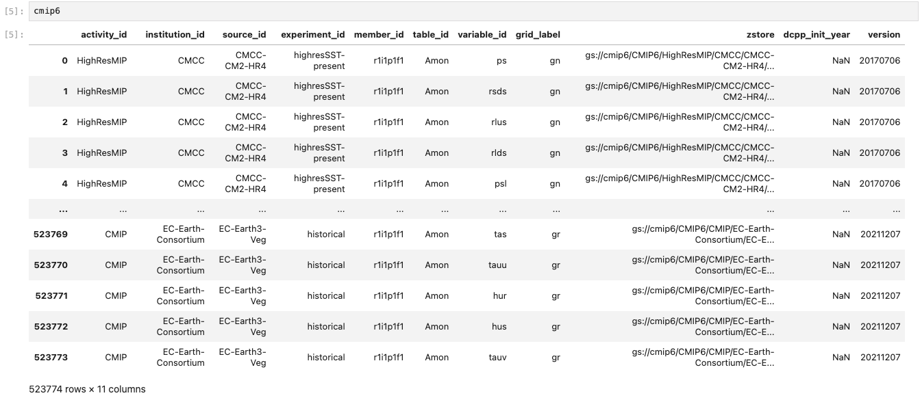
In the following sections, I’ll show you how to search for specific variables using metadata and efficiently compute different metrics from the data.
Global mean Sea Surface Temperature Changes
Let’s start with a simple example. The CMIP6 dataset includes a variable called tosga, which stands for Global Average Sea Surface Temperature. You can browse the full list of available variables in the official CMIP6 MIP tables.
To begin, we’ll extract the metadata—including the file locations—for the monthly mean tosga variable from the CMIP6 archive stored on Google Cloud. We can do this by…
# Query for all the historical data for the global mean SST
hist_files = cmip6.query("table_id == 'Omon' & variable_id == ['tosga'] \
                    & experiment_id ==['historical'] & member_id == ['r1i1p1f1']")
The list would look like this; 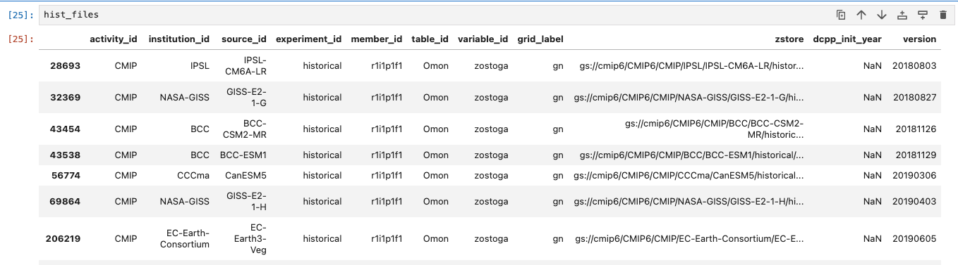
Similarly, extract the data for SSP 5-8.5, which is a high emission scenario.
ssp_files = cmip6.query("table_id == 'Omon' & variable_id == ['tosga'] \
                    & experiment_id ==['ssp585'] & member_id == ['r1i1p1f1']")
Now let’s select those CMIP6 models that have data for historical experiment and future scenarios. This will help us plot a continuous time series.
# Obtain available model names for historical dataset
hist_models = np.unique(hist_files['source_id'])
# Obtain available model names for SSP-5 8.5 dataset
ssp_models = np.unique(ssp_files['source_id'])
# Select models that are present in both Historical and SSP5-8.5 experiments
model_names = list(set(ssp_models) & set(hist_models))
Now that we have the list of models, let’s move on to extracting the data. In the next step, we’ll loop through each model, read both the historical data (1850–2014) and the SSP5-8.5 scenario data (2015–2100), and calculate the annual mean values. After extracting the datasets, we’ll combine them along the time dimension to create a continuous record from 1850 to 2100.
combined_data = []
for i in tqdm(range(len(model_names))):
    # Read the historical data and compute the annual mean
    hist_data = xr.open_zarr(hist_files[hist_files['source_id']\
                ==model_names[i]]['zstore'].item())['tosga'].groupby('time.year').mean('time')
    # Read the SSP 5-8.5 scenario data
    ssp_data = xr.open_zarr(ssp_files[ssp_files['source_id']\
                ==model_names[i]]['zstore'].item())['tosga'].sel(time=slice('2015-01-01','2100-12-31'))\
                .groupby('time.year').mean('time')
    # Combine along the time dimension and compute the annual mean
    combined_data.append(xr.concat([hist_data,ssp_data],dim='year'))
Pro Tip
Before running the full loop, it’s a good idea to test everything with just one model. This way, you can check that the data extraction and calculations are working correctly. Once everything looks good, you can expand the loop to include all the models.
To make computations easier later on, we’ll add the model information directly into the combined dataset. Thanks to how xarray is designed, it won’t immediately load all the actual data into memory when we read the files. Instead, it performs what’s called lazy loading—meaning only the metadata and coordinates are loaded at first. The full data will only be read into memory when we explicitly request it (for example, during computations or plotting).
# Combine the data for all CMIP6 models and load the data
cmip_data = xr.concat(combined_data,dim='models').load()
# Add the model name information
cmip_data = cmip_data.assign_coords({'models':model_names})
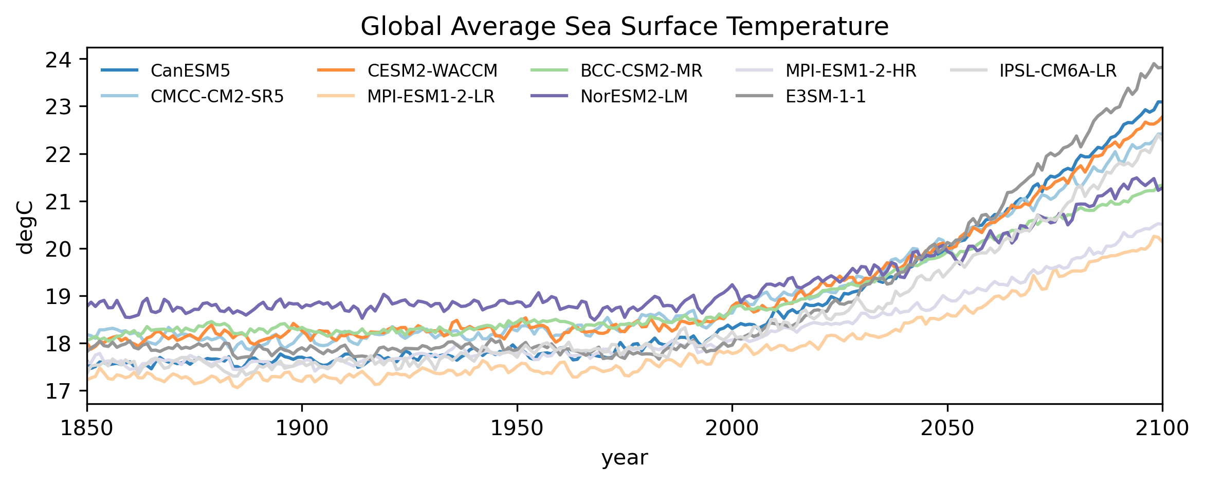
Finally, let’s plot the values.
# Divide the colors in the tab20c colorscheme into the length of models
colors = plt.cm.tab20c(np.linspace(0, 1, len(cmip_data.models.values)))
models = cmip_data.models.values

fig,ax = plt.subplots(1,1, figsize=(9,3),dpi=300)
# Loop through each model and plot data
for m in range(len(cmip_data.models.values)):
    ((cmip_data.sel(models=models[m])))\
            .plot(ax=ax,label=models[m],c=colors[m],alpha=1)
# Set the proper limits along X-axis
ax.set_xlim(cmip_data['year'].values[0],cmip_data['year'].values[-1])
ax.set_ylabel('degC')
ax.legend(ncols=5,loc='upper left',fontsize=8,frameon=False)
ax.set_title('Global Average Sea Surface Temperature')
plt.show()
Compute El Niño Southern Oscillation Present and Future
The El Niño Southern Oscillation (ENSO) is one of the most influential modes of climate variability, significantly affecting weather and rainfall patterns across the globe. To quantify ENSO, we usually calculate an index based on the anomalous area-averaged sea surface temperature (SST) over the Niño 3.4 region (located roughly between 5°N–5°S latitude and 170°W–120°W longitude).
Unlike the previous example where we worked with a pre-computed global average, in this case, we need to extract and calculate the ENSO index directly from global SST data. The good news is: we don’t need to download entire datasets to do this. Instead, we can compute the Niño 3.4 average for each time step directly during the data reading process.v To make this process efficient, we’ll define a simple function that:
- Reads the global surface temperature field,
- Selects the Niño 3.4 region,
- Calculates the area-weighted average. Let’s define the function next!
def extract_index(ds):
    '''
    The function takes CMIP6 data as input and calculate the area averaged value of
    surface temperature over the Nino 3.4 region.
    '''
    nino34_ts = ds['ts'].sel(lat=slice(-5,5),lon=slice(190,240)).load()
    nino34_ts = nino34_ts.weighted(np.cos(nino34_ts['lat']*np.pi/180))\
            .mean(dim=('lon','lat'))
    return nino34_ts
Next, we’ll retrieve all available data for monthly mean surface temperature (ts) over the Niño 3.4 region from both the historical (1850–2014) and SSP5-8.5 (2015–2100) datasets and combine them as we did before.
# Search for historical datasets
hist_files = cmip6.query("table_id == 'Amon' & variable_id == ['ts'] \
                    & experiment_id ==['historical'] & member_id == ['r1i1p1f1']")
# Search for SSP-5 8.5 datasets
ssp_files = cmip6.query("table_id == 'Amon' & variable_id == ['ts'] \
                    & experiment_id ==['ssp585'] & member_id == ['r1i1p1f1']")

ssp_models = np.unique(ssp_files['source_id'])
hist_models = np.unique(hist_files['source_id'])
model_names = sorted(list(set(ssp_models) & set(hist_models)))

combined_data = []
for i in tqdm(range(len(model_names))):
    # Read historical data
    hist_data = xr.open_zarr(hist_files[hist_files['source_id']\
                ==model_names[i]]['zstore'].item())
    # Redefine the time axis. Helps with merging.
    histime = xr.cftime_range(start='1850-01-01',freq='1MS',periods=len(hist_data['time']))
    hist_data = hist_data.assign_coords({'time':histime})\
                .sel(time=slice('1850-01-01','2014-12-31'))
    # Extract ENSO TAS
    hist_nino = extract_index(hist_data)
    # Read SSP5-8.5 data
    ssp_data = xr.open_zarr(ssp_files[ssp_files['source_id']\
                    ==model_names[i]]['zstore'].item())
    # Redefine the time axis. Helps with merging.
    ssptime = xr.cftime_range(start='2015-01-01',freq='1MS',periods=len(ssp_data['time']))
    ssp_data = ssp_data.assign_coords({'time':ssptime})\
                .sel(time=slice('2015-01-01','2099-12-31'))
    # Extract ENSO TAS
    ssp_nino = extract_index(ssp_data)
    # Combine the historical and future timeseries
    combined_data.append(xr.concat([hist_nino,ssp_nino],dim='time'))

# Combine and add the models as another coordinate
cmip_data = xr.concat(combined_data,dim='models').assign_coords({'models':model_names})
Next step is to calculate the anomaly with respect to a reference period to obtain the ENSO index.
# Reference period to calculate mean climatology
refperiod = slice('1850-01-01','1949-12-31')
# Calcualate temperature anomaly
nino_anom = cmip_data.groupby('time.month') - cmip_data.sel(time=refperiod)\
                                .groupby('time.month').mean('time')
# Detrend to obtain the ENSO Index
nino_index = xr.apply_ufunc(polynomial_detrend,nino_anom,\
            vectorize=True,input_core_dims=[['time']],\
            output_core_dims=[['time']])
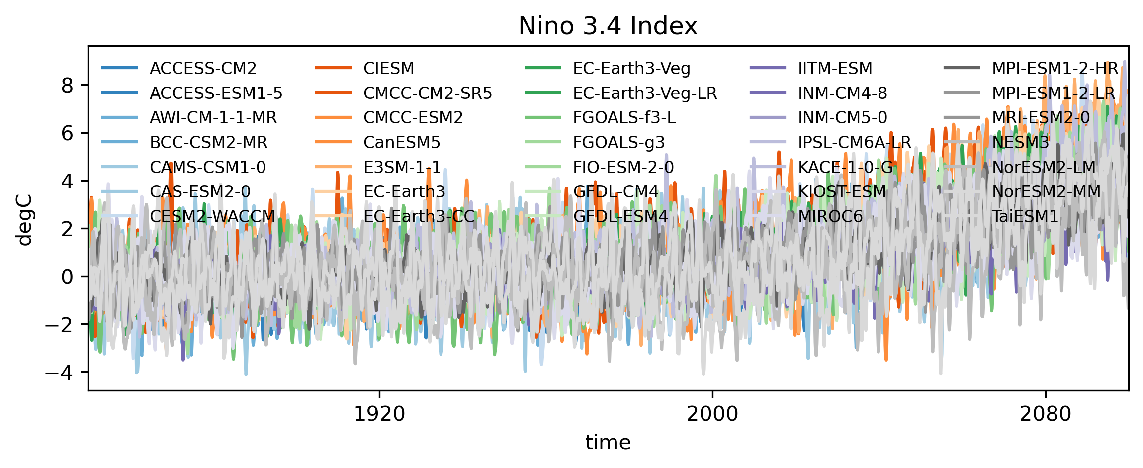
Now finally let’s plot the data.
# Divide the colors in the tab20c colorscheme into the length of models
colors = plt.cm.tab20c(np.linspace(0, 1, len(cmip_data.models.values)))
models = cmip_data.models.values

fig,ax = plt.subplots(1,1, figsize=(9,3),dpi=300)
# Loop through each model and plot data
for m in range(len(cmip_data.models.values)):
    ((nino_anom.rolling(time=3,center=True).mean('time').sel(models=models[m])))\
            .plot(ax=ax,label=models[m],c=colors[m],alpha=1)
ax.set_title('Nino 3.4 Index')
ax.set_ylabel('degC')
ax.set_xlim(cmip_data['time'].values[0],cmip_data['time'].values[-1])
ax.legend(ncols=5,loc='upper left',fontsize=8,frameon=False)
plt.show()
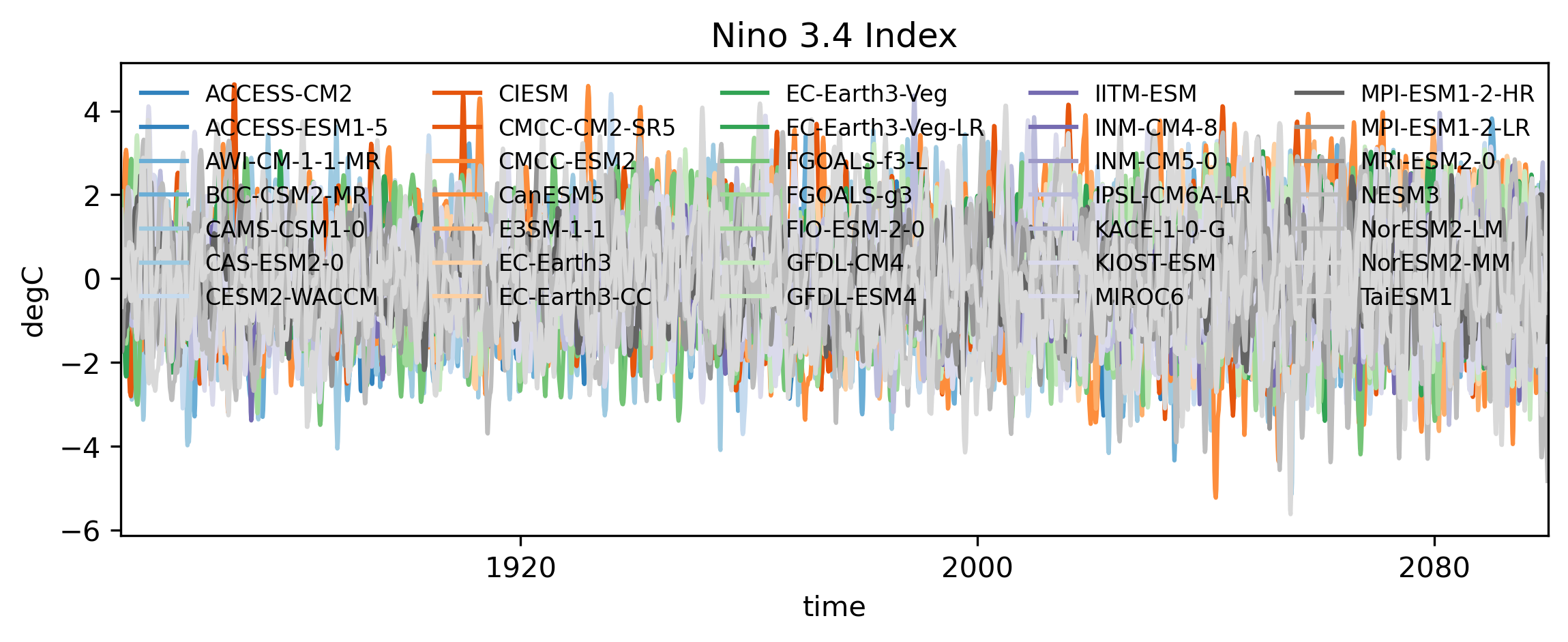
Optionally, we can detrend the surface temperature anomalies to remove the underlying long-term warming trend caused by climate change. This step isolates the natural variability, like ENSO, from the background global warming signal. A simple way to do this is by fitting and removing a 4th-order polynomial trend from the time series. This captures the gradual, monotonic increase without affecting the interannual variability. Let’s define a function that applies this detrending:
def polynomial_detrend(data):
    '''
    Apply a 4th order polynomial detrending
    '''
    pcoef = np.polyfit(np.arange(len(data)),data,deg=4)
    ptrend = np.polyval(pcoef.T,np.arange(len(data)))
    return data-ptrend
The detrending function can now be applied directly to your time series. Here’s how you can use it:
# Reference period to calculate mean climatology
refperiod = slice('1850-01-01','1949-12-31')
# Calcualate temperature anomaly
nino_anom = cmip_data.groupby('time.month') - cmip_data.sel(time=refperiod)\
                                .groupby('time.month').mean('time')
# Detrend to obtain the ENSO Index
nino_index = xr.apply_ufunc(polynomial_detrend,nino_anom,\
            vectorize=True,input_core_dims=[['time']],\
            output_core_dims=[['time']])
Finally, let’s plot the Niño 3.4 index to see how it looks—both with detrending:
colors = plt.cm.tab20c(np.linspace(0, 1, len(cmip_data.models.values)))
models = cmip_data.models.values

fig,ax = plt.subplots(1,1, figsize=(9,3),dpi=300)
for m in range(len(cmip_data.models.values)):
    ((nino_index.rolling(time=3,center=True).mean('time').sel(models=models[m])))\
            .plot(ax=ax,label=models[m],c=colors[m],alpha=1)
ax.set_title('Nino 3.4 Index')
ax.set_ylabel('degC')
ax.set_xlim(cmip_data['time'].values[0],cmip_data['time'].values[-1])
ax.legend(ncols=5,loc='upper left',fontsize=8,frameon=False)
plt.show()
Future rainfall changes over North America
Precipitation is one of the most important variables in global climate model (GCM) simulations. It is a key driver for understanding climate impacts on ecosystems, agriculture, and water resources. In this section, we’ll also get hands-on experience working with a truly multidimensional variable. Our goal will be to retrieve precipitation data (pr) from all available CMIP6 models. However, to perform a meaningful model intercomparison, we need all the datasets to be on the same grid. Different GCMs often use different native resolutions, so we will regrid (interpolate) the precipitation data to a common grid resolution.
As in the previous examples, we’ll start by selecting the right variable—in this case, monthly precipitation (pr). We’ll read in precipitation data from two experiments-the historical experiment (1850–2014), and the SSP5-8.5 future scenario (2015–2100). Then, we’ll filter and retain only the models that provide data for both experiments, ensuring consistency across our analysis.
hist_files = cmip6.query("table_id == 'Amon' & variable_id == ['pr'] \
                    & experiment_id ==['historical'] & member_id == ['r1i1p1f1']")
ssp_files = cmip6.query("table_id == 'Amon' & variable_id == ['pr'] \
                    & experiment_id ==['ssp585'] & member_id == ['r1i1p1f1']")
ssp_models = np.unique(ssp_files['source_id'])
hist_models = np.unique(hist_files['source_id'])
model_names = list(set(ssp_models) & set(hist_models))
There are several methods available for interpolating climate model data onto a common grid, ranging from simple linear interpolation to more sophisticated conservative remapping techniques. For this tutorial, we will keep things simple and use a basic function that takes two Xarray DataArrays as inputs: it will interpolate the first dataset onto the grid of the second dataset.
Here’s how you can define the interpolation function:
def regrid_to_target(source_da, target_da):
    """
    Interpolates the source DataArray onto the grid of the target DataArray.

    Parameters:
    - source_da: xarray.DataArray
        The dataset you want to interpolate.
    - target_da: xarray.DataArray
        The dataset providing the target grid (lat/lon).

    Returns:
    - xarray.DataArray
        The interpolated dataset.
    """
  return source_da.interp_like(target_da)
To ensure that all precipitation datasets are on the same spatial grid, we first need a target grid for interpolation. We can easily create a dummy dataset that defines the desired grid. Here’s an example:
# Make a sample dataset to which you want to interpolate the data.
# You can also load a dataset
lon = np.arange(0,360,2.5)
lat = np.arange(-90,91,2.5)
dummy_data = np.zeros([len(lon),len(lat)])
target_grid = xr.DataArray(dummy_data,coords={'lon':lon,'lat':lat})
Now that we have our reference grid set up, let’s move forward: We’ll loop through each available model, extract the precipitation data over the North America region, and interpolate it onto the common 2.5° x 2.5° grid we defined earlier.
An important advantage of this approach is efficiency: At any given time, we will only load data from a single model and only for the North American region. This means we don’t need to download or keep the full global precipitation dataset for all models in memory—greatly reducing the memory footprint of our analysis and making it manageable even on modest computing setups.
In short, we’ll work smart by:
- Reading one model at a time
- Subsetting to just the North America region
- Interpolating immediately onto the common grid
- Combining the processed outputs
# Latitudinal Box for North America
latslice = slice(0,90)
# Longitudinal Box for North America
lonslice = slice(180,360)

combined_data = []
for i in tqdm(range(len(model_names))):
    # Read Historical Data
    hist_data = xr.open_zarr(hist_files[hist_files['source_id']\
                ==model_names[i]]['zstore'].item())['pr']
    # Redefine historical time range to make sure all models have same time axis
    histime = xr.cftime_range(start='1850-01-01',freq='1MS',periods=len(hist_data['time']))
    hist_data = hist_data.assign_coords({'time':histime})\
                .sel(time=slice('1850-01-01','2015-12-31'))
    hist_idata = regrid_to_target(hist_data.sel(lat=latslice,lon=lonslice),\
                          odata.sel(lat=latslice,lon=lonslice))

    ssp_data = xr.open_zarr(ssp_files[ssp_files['source_id']\
                    ==model_names[i]]['zstore'].item())['pr']
    # Redefine SSP time range to make sure all models have same time axis
    ssptime = xr.cftime_range(start='2015-01-01',freq='1MS',periods=len(ssp_data['time']))
    ssp_data = ssp_data.assign_coords({'time':ssptime})\
                .sel(time=slice('2016-01-01','2099-12-31'))
    ssp_idata = regrid_to_target(ssp_data.sel(lat=latslice,lon=lonslice),\
                        odata.sel(lat=latslice,lon=lonslice))
    # Combine the data along time dimension
    combined_data.append(xr.concat([hist_idata,ssp_idata],dim='time'))
# Add model information
cmip_data = xr.concat(combined_data,dim='models').assign_coords({'models':model_names})
Now that we have all our precipitation data extracted, interpolated, and ready, it’s time to move to the analysis stage. We will split the combined dataset into three different time periods and calculate the seasonal mean precipitation for each period separately. The time periods we’ll use are:
- Historical: 1980–2009
- Present-Day / Near-Future: 2011–2040
- Far-Future: 2070–2099
# Historical period
hslice = slice('1980-01-01','2009-12-31')
# Present period
pslice = slice('2011-01-01','2040-12-31')
# Future period
fslice = slice('2070-01-01','2099-12-31')

# Calculate historical climatology
hclim = cmip_data.sel(time=hslice).groupby('time.season').mean('time')
# Calculate present climatology
pclim = cmip_data.sel(time=pslice).groupby('time.season').mean('time')
# Calculate future climatology
fclim = cmip_data.sel(time=fslice).groupby('time.season').mean('time')
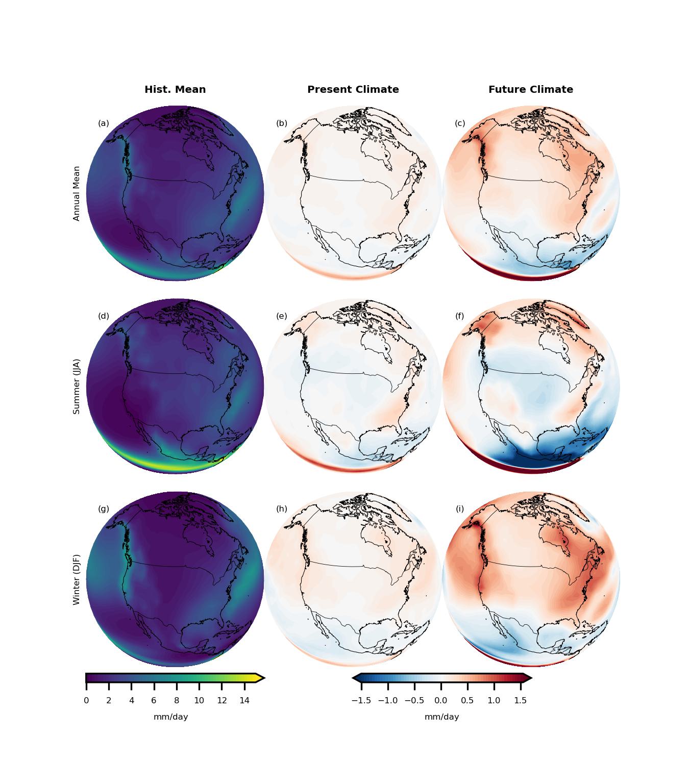
By comparing the seasonal means across these periods, we can observe how precipitation patterns are projected to evolve over North America under the high-emission SSP5-8.5 scenario. Finally, let’s bring all of this together and visualize the results! We’ll create some clear, informative plots to show how precipitation patterns change over time across the North American continent.
Time to make some pretty maps and really see the story the models are telling us!
plt.rcParams.update({'font.size': 4})
fig,ax = plt.subplots(3,3,figsize=(4.5,5),dpi=300,frameon=False,\
            subplot_kw={'projection':ccrs.NearsidePerspective(central_longitude=260.0,\
                        central_latitude=45.0, satellite_height=4e6)})
                               central_latitude=50)})
ax=ax.flatten()
plotd = [hclim.mean(dim=('models','season')),\
        (pclim-hclim).mean(dim=('models','season')),\
        (fclim-hclim).mean(dim=('models','season')),\
        hclim.sel(season='JJA').mean('models'),\
        (pclim-hclim).sel(season='JJA').mean('models'),\
        (fclim-hclim).sel(season='JJA').mean('models'),\
        hclim.sel(season='DJF').mean('models'),\
        (pclim-hclim).sel(season='DJF').mean('models'),\
        (fclim-hclim).sel(season='DJF').mean('models')]
levs = [np.arange(0,15.1,.25),np.arange(-1.5,1.6,.05),np.arange(-1.5,1.6,.05)]*3
# levs = [np.arange(0,15.1,1),np.arange(-1.5,1.6,.5),np.arange(-1.5,1.6,.5)]*3
titles = ['Hist. Mean', 'Present Climate', 'Future Climate']
pl = []
for a in range(len(ax)):
    pl.append((plotd[a]*86400).plot.contourf(ax=ax[a],transform =ccrs.PlateCarree(),\
                    add_colorbar=False,levels=levs[a]))
    t_pos = ax[a].get_position()
    ax[a].text(.1,.9,'({})'.format(ascii_lowercase[a]),\
               transform=ax[a].transAxes,va='center',ha='center')
    # ax[a].text(190,65,'({})'.format(ascii_lowercase[a]),transform =ccrs.PlateCarree())
    ax[a].coastlines(lw=.25,resolution='50m')
    ax[a].add_feature(cfeature.BORDERS,lw=.2)
    ax[a]._frameon = False
    ax[a].set_title('')
plt.subplots_adjust(wspace=0, hspace=-.05)
for a in range(3):
    ax[a].set_title(titles[a],fontweight='bold')
stitles = ['Annual Mean','Summer (JJA)','Winter (DJF)']
for a in np.arange(0,len(ax),3):
    ax[a].text(-0.05,.5,stitles[a//3],transform=ax[a].transAxes,\
              rotation=90,va='center',ha='center')

cb_pos = ax[-3].get_position()
pos_cax= fig.add_axes([cb_pos.x0,cb_pos.y0-.02,\
                       cb_pos.width,cb_pos.height/20])
cb=plt.colorbar(pl[0], cax=pos_cax, orientation='horizontal', ticks=levs[0][::8])
cb.minorticks_off()
cb.set_label('mm/day')
cb_pos = ax[-1].get_position()
pos_cax= fig.add_axes([cb_pos.x0-cb_pos.width/2,cb_pos.y0-.02,\
                       cb_pos.width,cb_pos.height/20])
cb=plt.colorbar(pl[-1], cax=pos_cax, orientation='horizontal', ticks=levs[-1][::10])
cb.minorticks_off()
cb.set_label('mm/day')